Supplementary web page to the paper
The above-titled paper was presented at EUSIPCO 2014 conference. The paper is available here. This webpage serves as supplementary to this paper, in sense of the reproducible research idea.
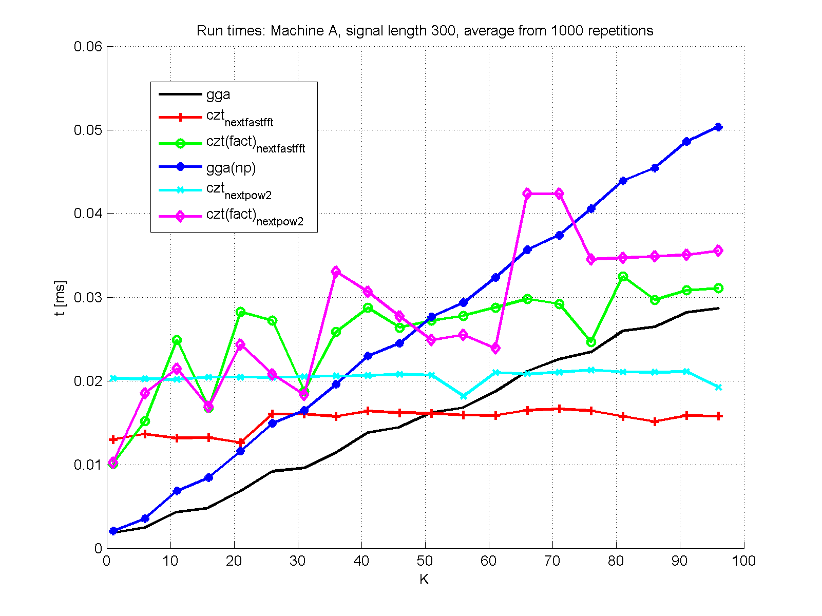
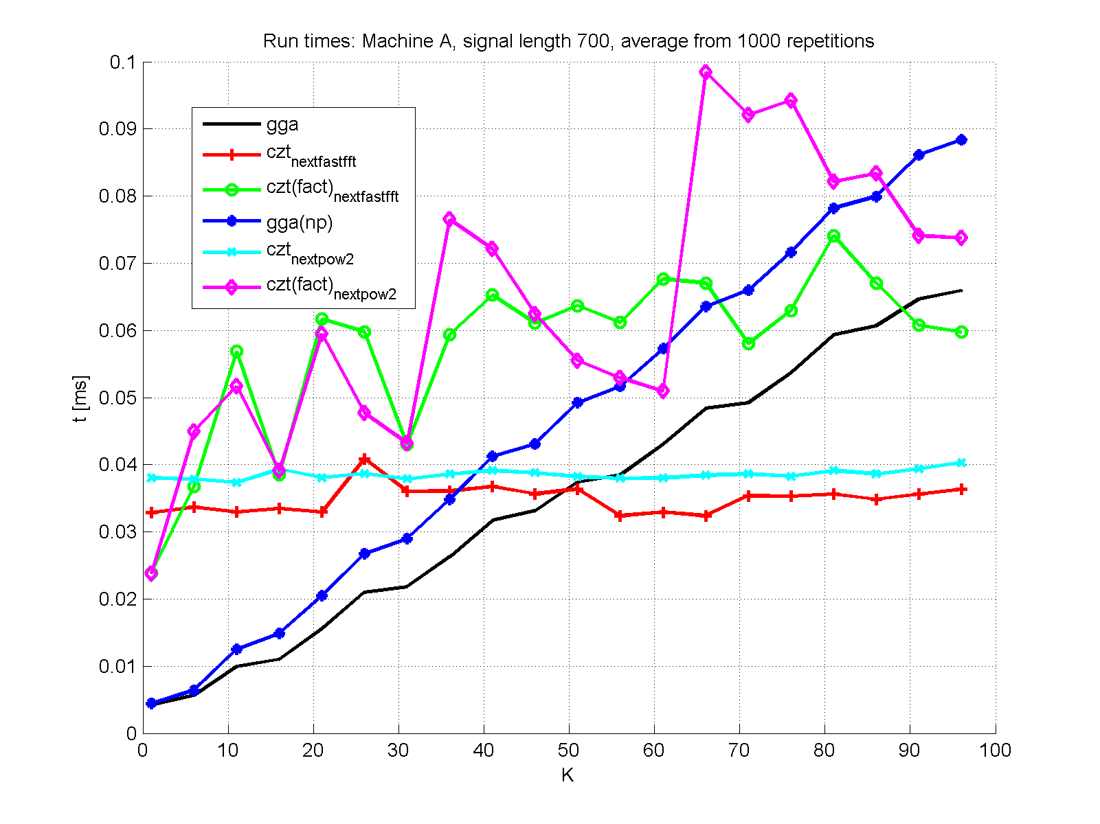
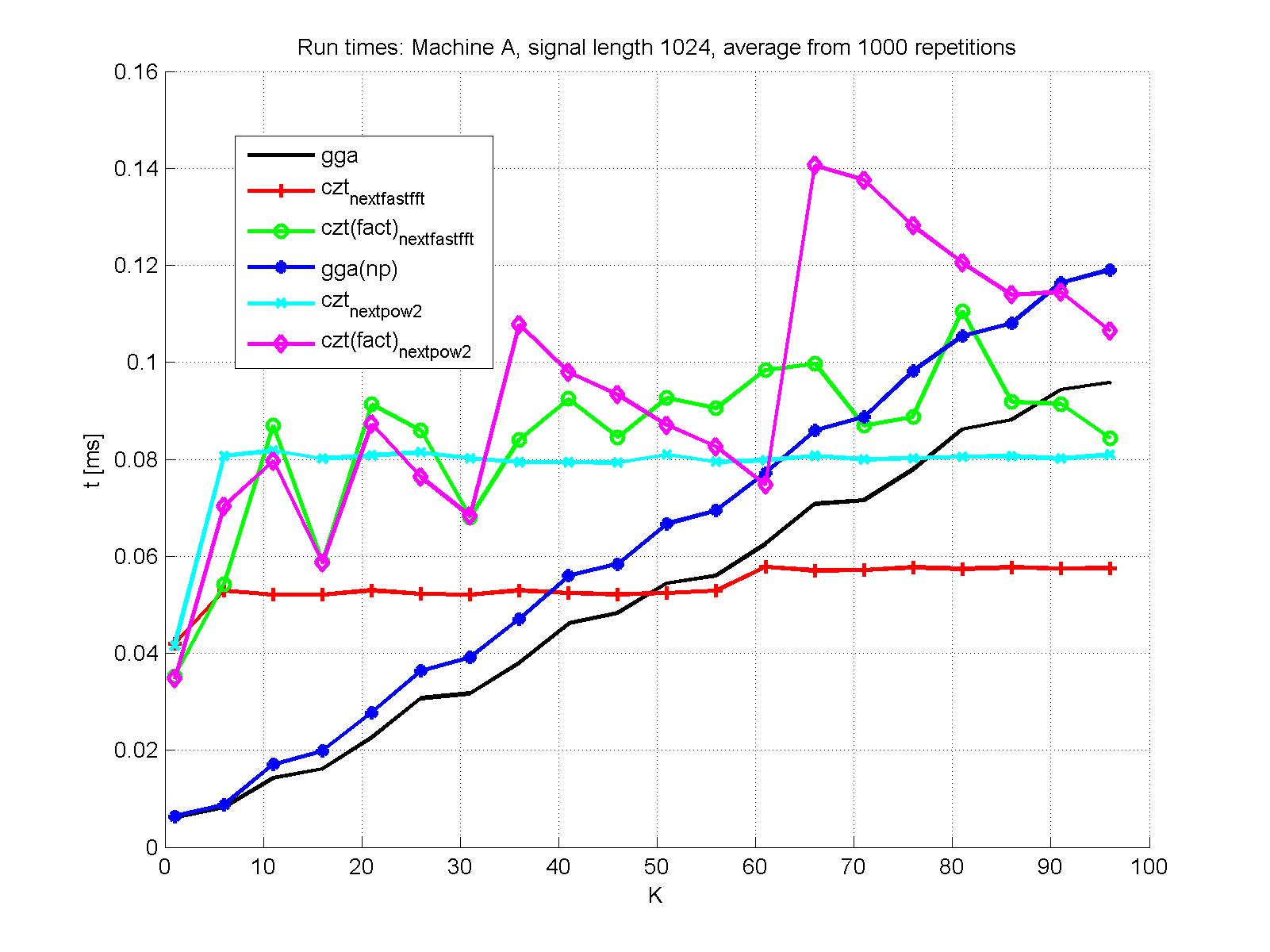
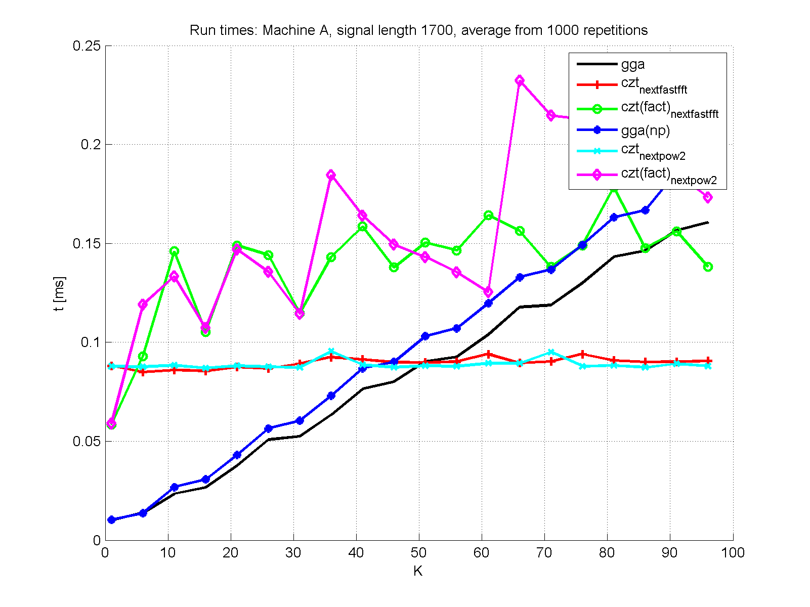
We take the two natural competitors in the area of fine-scale spectrum analysis, namely the Chirp Z-transform (CZT) and the Generalized Goertzel algorithm (GGA), and compare the two, focusing on the computational cost point of view. We present results that favor the GGA over the CZT in many practical situations, in terms of complexity for real-input data. This is shown both in theory and in practice.
The computational costs of the CZT and the GGA are compared also practically in the paper. The basic procedure and tested algorithms are described in the paper. We give some more details here.
The measuring batch has to be run from Matlab, which, however, serves just to run the appropriate commands and then collect and save measured data. In turn, MATLAB version does not play a role.
This archive contains all files necessary files for reproducing our plots or/and perform your own measurement. The archive is divided into folders:
measure/..............................Files
for performing the
tests. The main file is time_ggavsczt.m. The folder then contains DLL
libraries of FFTW and LTFAT, as well as the executables, compiled
for 64bit Windows. Such users can therefore perform their own
measurement just by running the main file from Matlab.
src/.....................................Source
codes for all the
algorithms in Matlab and of the timing executables in C. The C
implemetation of the algorithms is part of LTFAT
from ver. 1.4.3 upwards. If you wish to run your experiment on system
other than Win 64bit (including Unix-type systems), please see the
README file for compilation
instructions.
measured/..........................Measurement
results of a few
computers (see their specification below). Matlab MAT files.
graphic_comparison/.............Matlab
script taking the saved results
and plotting various graphs comparing the speed of the algorithms. Set
the booleans at the first few lines to choose what plots to show.
First, we present timing plots for Machine A for several signal lengths:
|
|
|
|
Now the same timings, measured at Machine C:
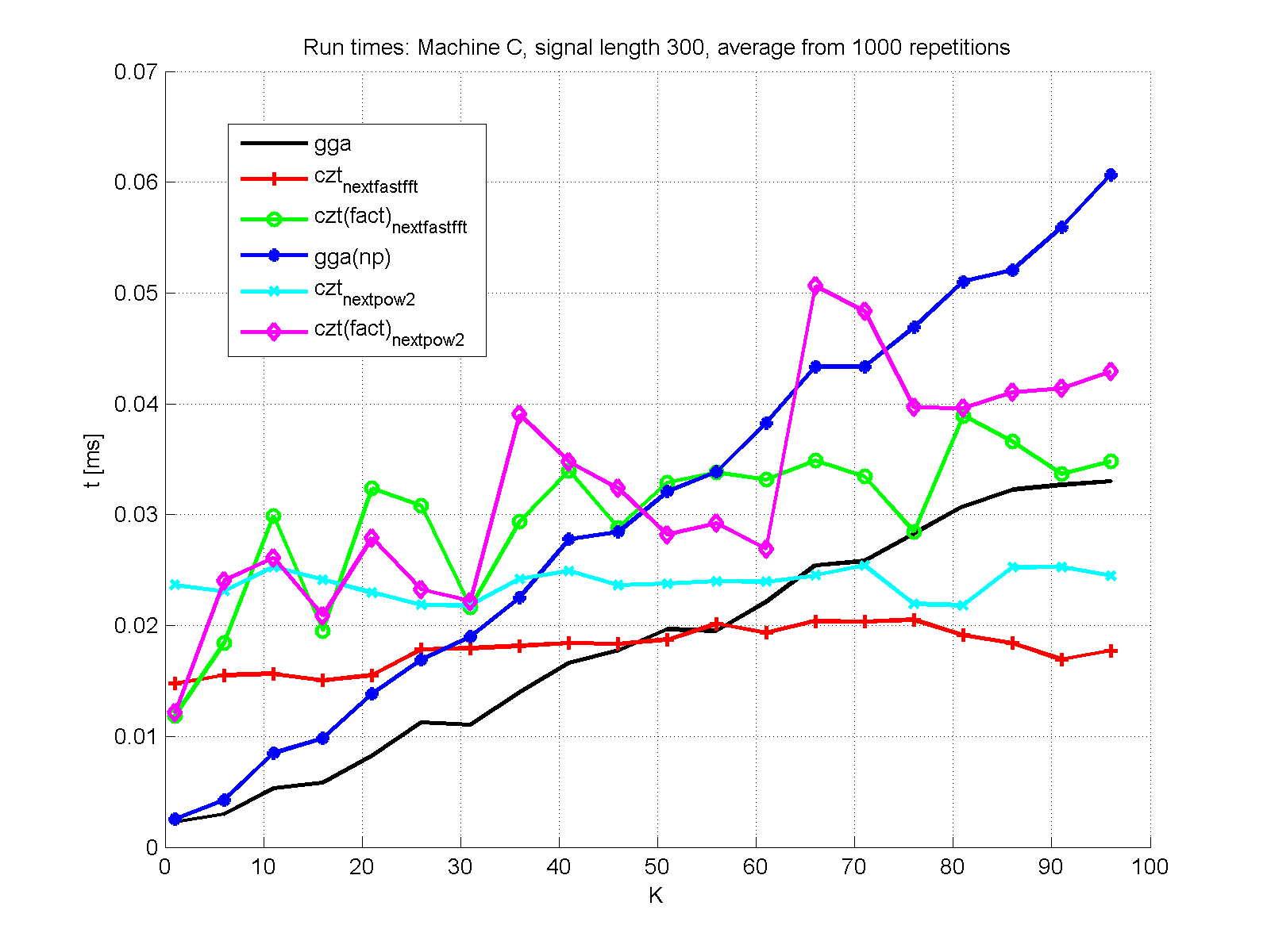 |
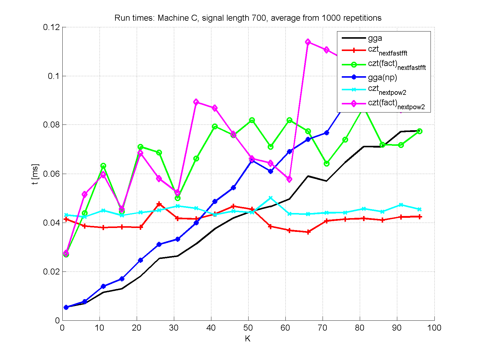 |
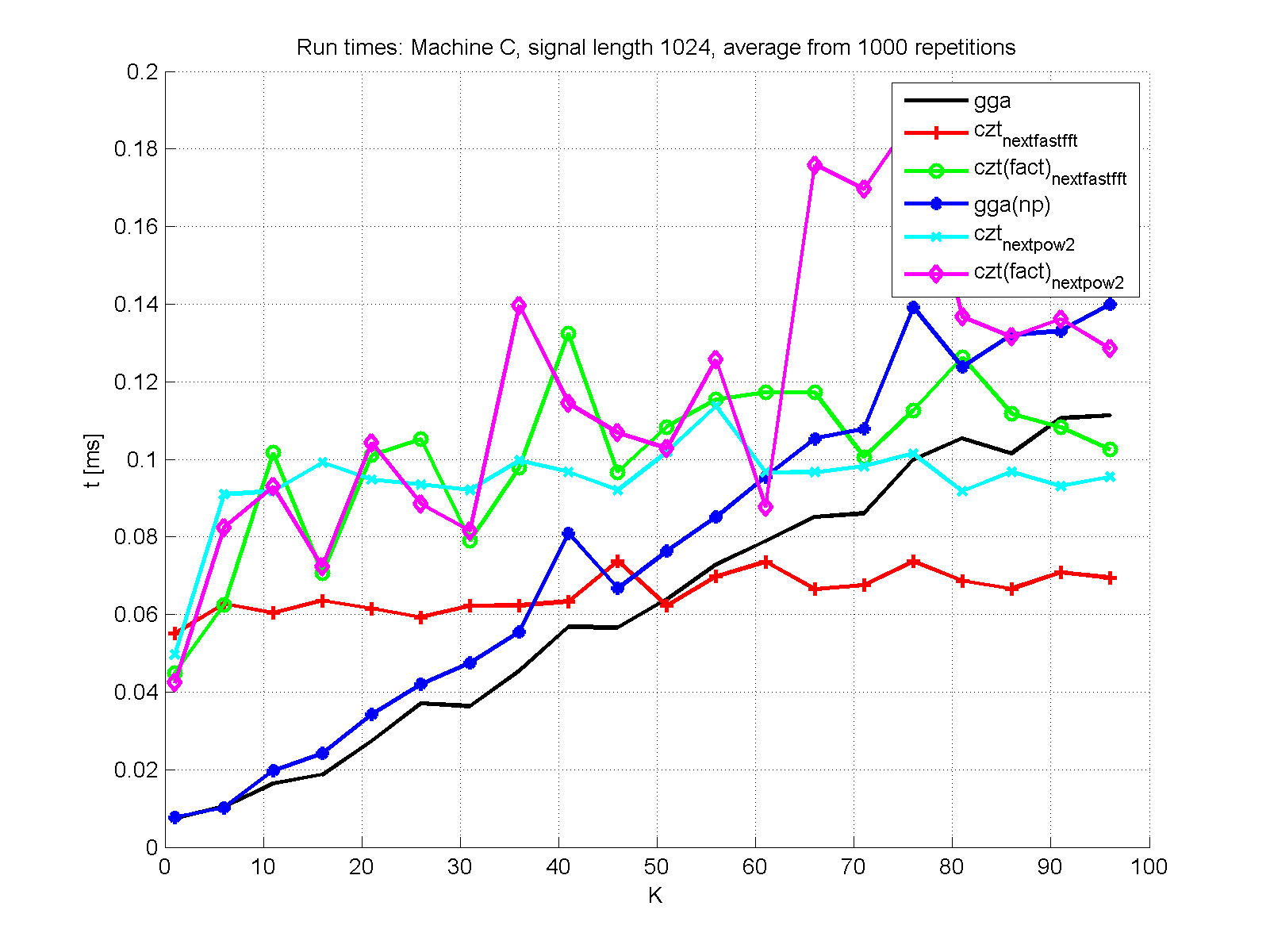 |
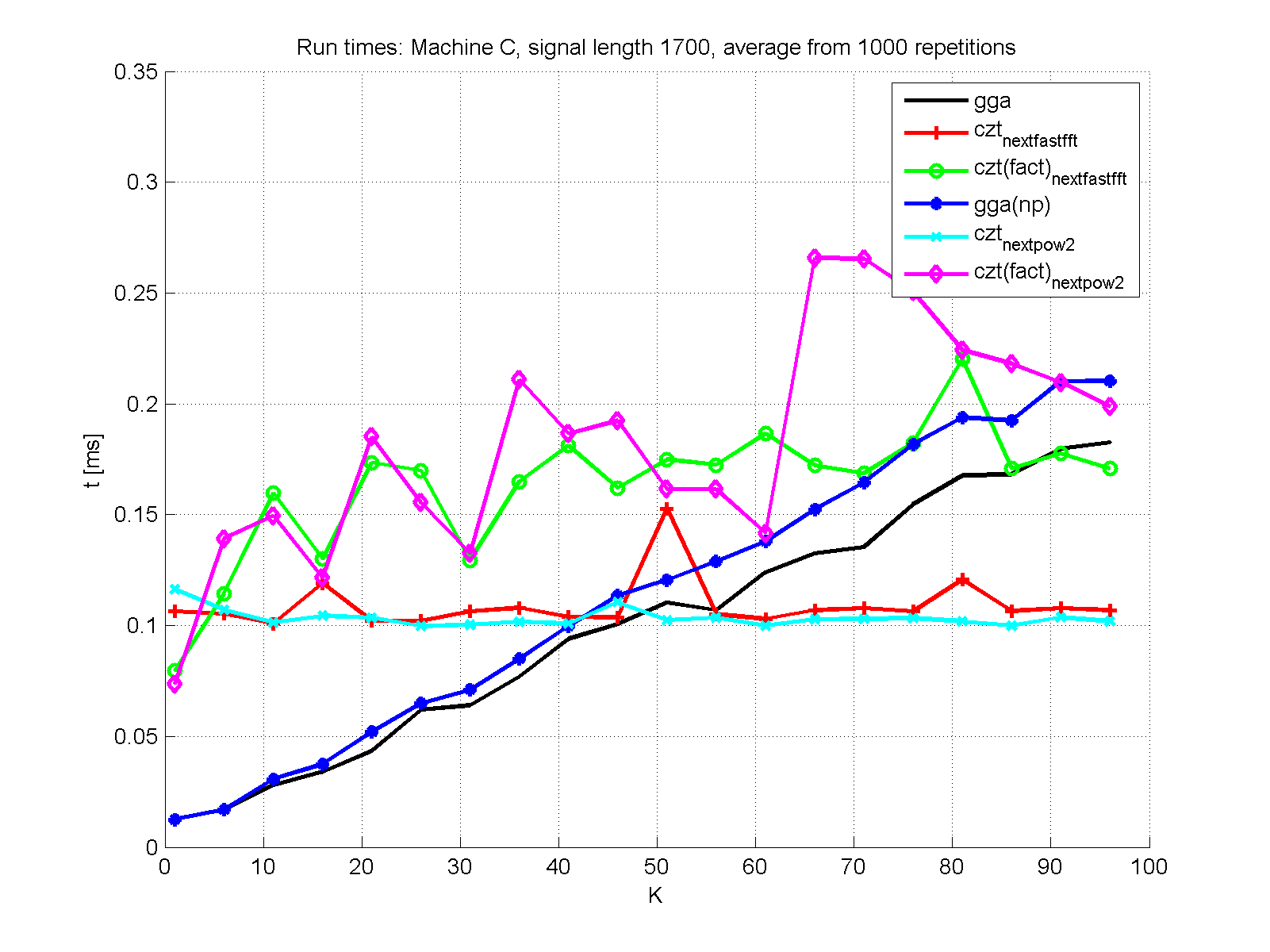 |
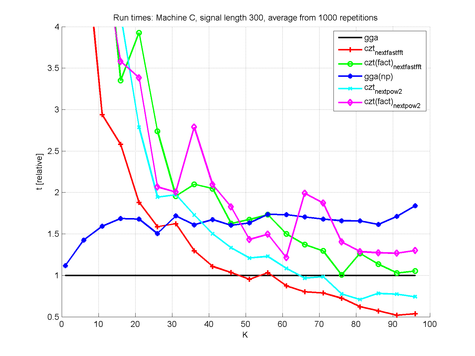
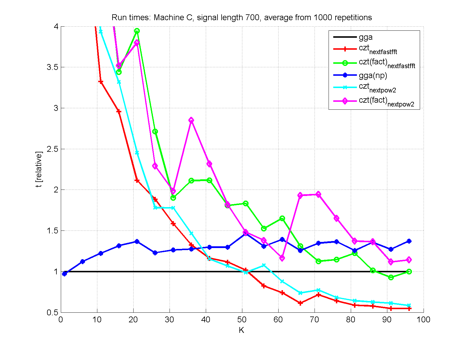
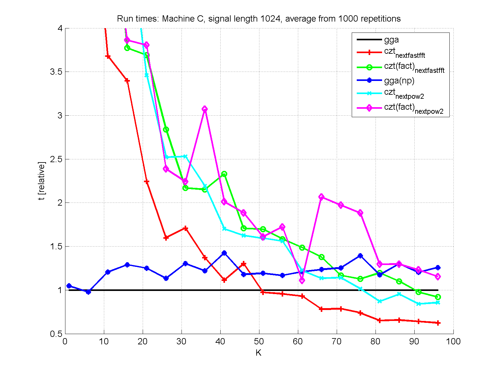
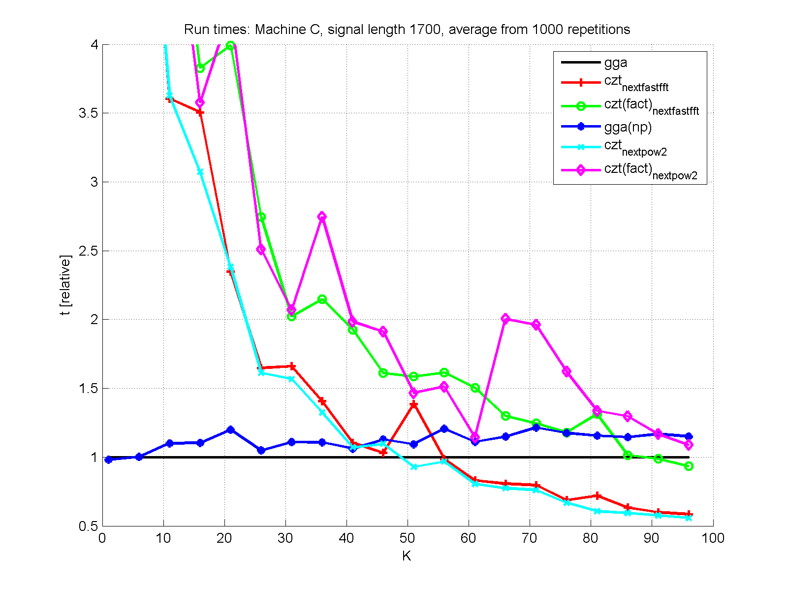
Next set is timing measured at Machine C, but this time relative to the GGA:
 |
 |
 |
 |
And finally, we present relative timings averaged over Machines A to F:
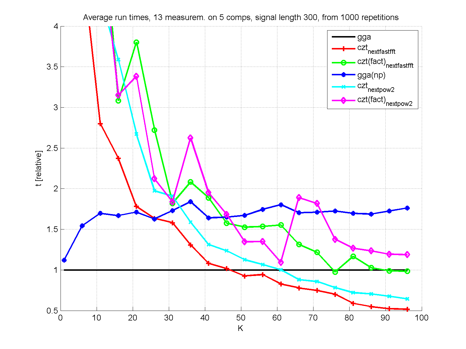 |
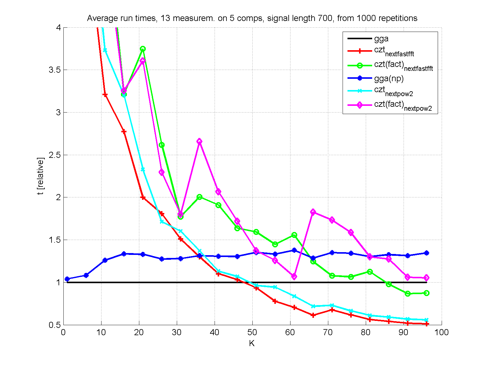 |
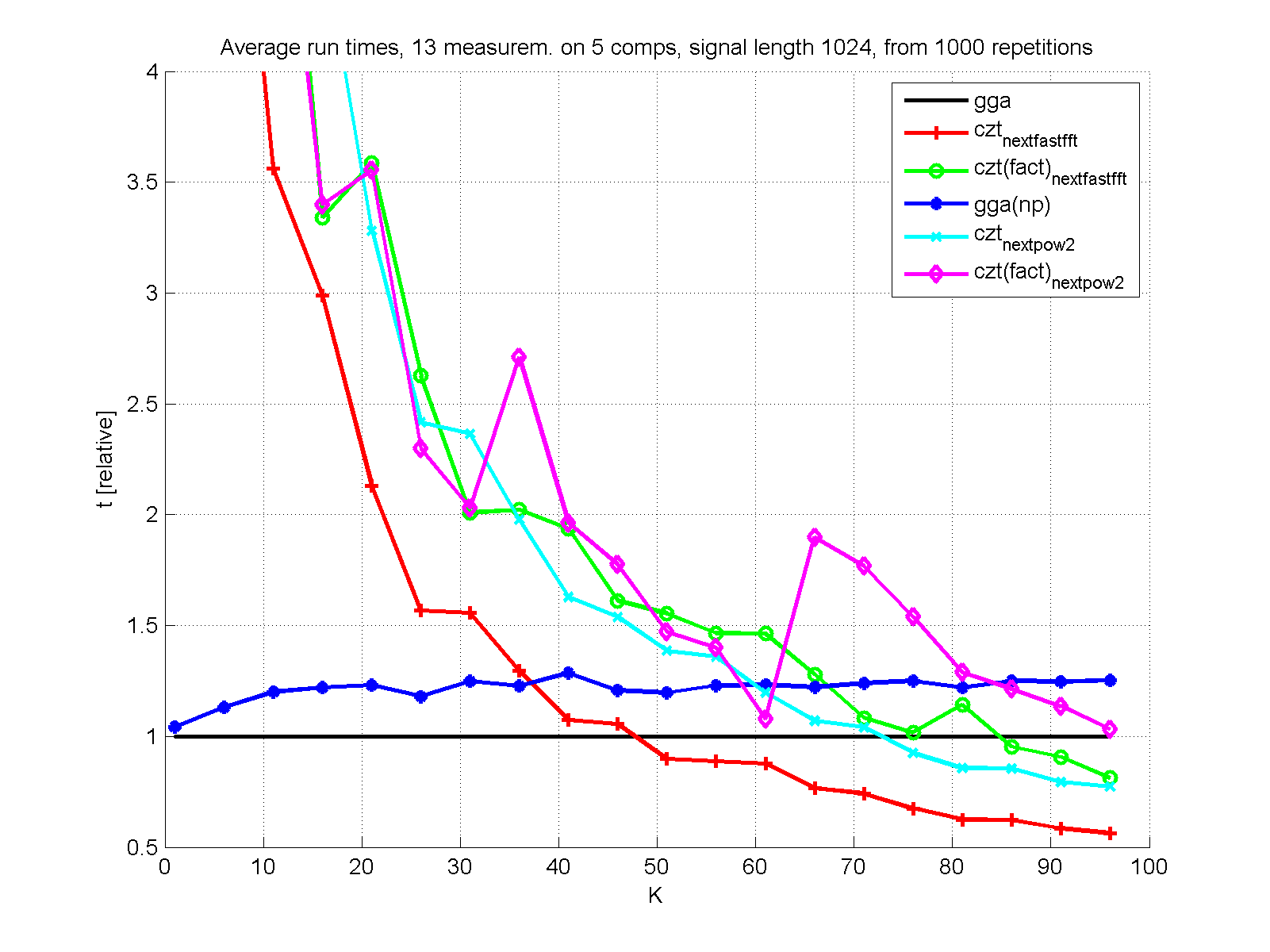 |
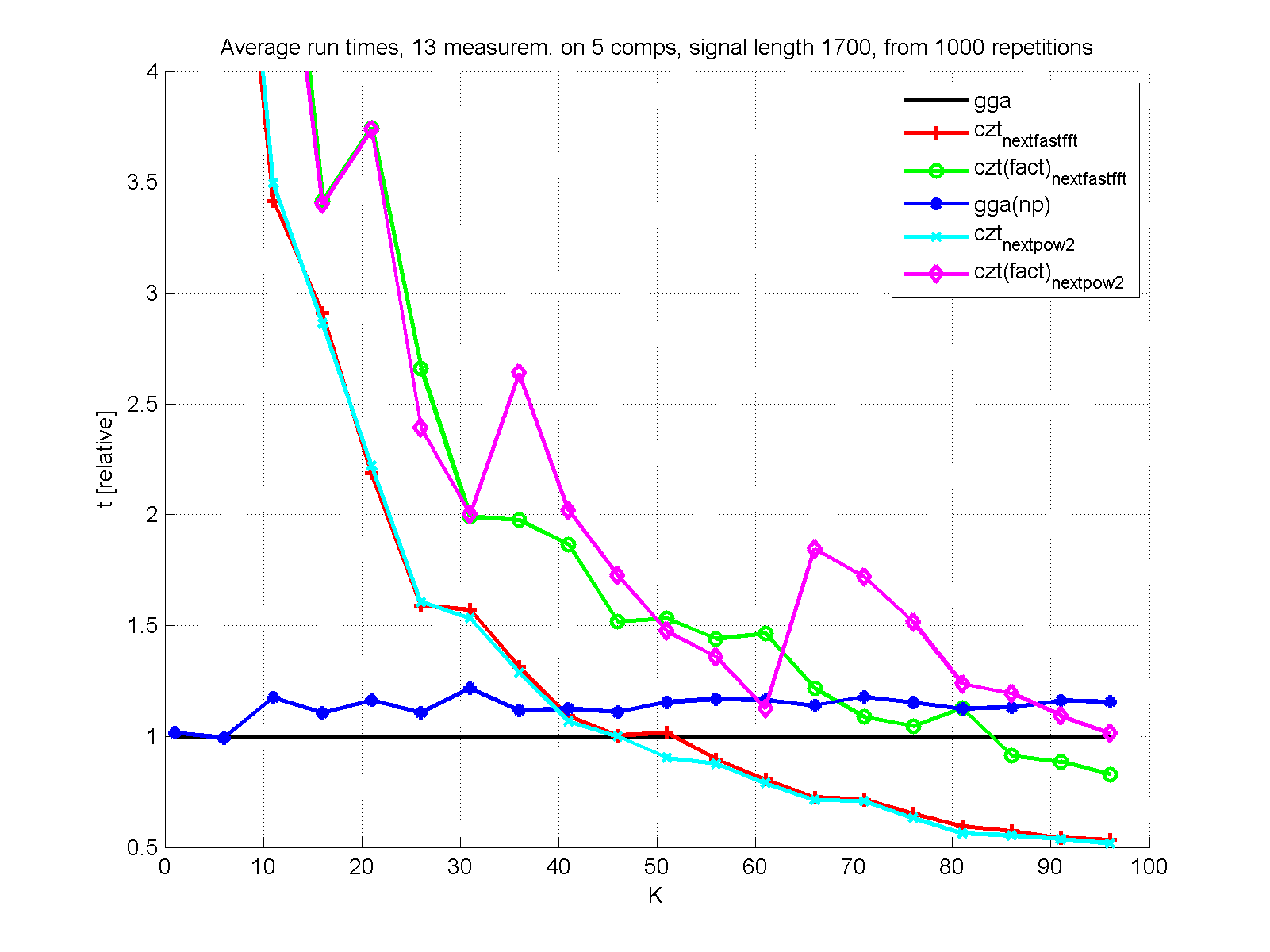 |
Specifications
of the measured
computers follow. The reproducibility of our results is not possible
here, of course; however we provide the measured data on these machines.
Machine A:
Desktop PC of ZP
file cztvsgga_25-Oct-2013_18-12-16-Prusa.mat
Intel(R) Core(TM)2 Quad CPU @ 2.40GHz
3GB memory
Windows 7 64bit
Machine B:
Desktop of VM
file cztvsgga_27-Oct-2013_07-55-17-Mach_PC_skolni.mat
Intel(R) Core(TM) i7 CPU 960 @ 3.20GHz
Windows 7 64bit
Machine C:
Notebook of VM
file cztvsgga_27-Oct-2013_07-51-33-Mach_notebook.mat
Intel(R) Core(TM)2 Duo CPU T5870 @ 2.00GHz
Windows 7 64bit
Machine D:
PC in laboratory SC5.113
files cztvsgga_29-Oct-2013_08-??-??-SC5.113.mat
Intel(R) Core(TM) i5 CPU 680 @ 3.60GHz
12GB memory
Windows 7 64bit
Machine E:
PC in laboratory SC5.127
files cztvsgga_01-Nov-2013_14-??-??-SC5.127.mat
Intel(R) Core(TM) i5 CPU 680 @ 3.60GHz
Windows 7 64bit